The Data collected by Tokeet throughout the day to day importing of bookings and guest information is not always in the form you need it to be to accomplish other important tasks. For example, a cleaning fee set on Booking.com will not show on your Inquiry Data feed unless you have added it directly to the booking in Tokeet.
For a detailed walk-through on how to download a data feed report please see the following guide.
This article aims to introduce some basic concepts that are useful when manipulating the data on a spreadsheet application like Excel or Google Sheets.
Using the Data in the *.CSV file in Excel
Double click the csv file to open it in Excel
To show all data fully in the columns, you will need to AutoFit columns
Start by selecting all data using the small square at the top left of your worksheet.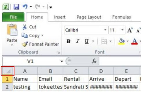
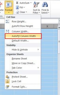
Go to Format > AutoFit Column Width. This will make all data visible within each column.
Applying filters to your spreadsheet is an important skill that allows you to view, alter, or add to specific rows that fall within the criteria of your filter selection.
To add a filter simply select the filter icon on the Data tab of Microsoft Excel.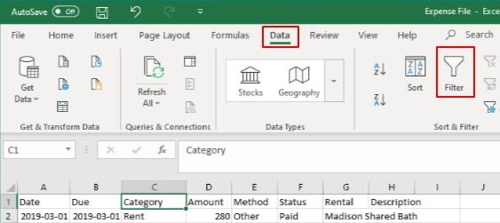
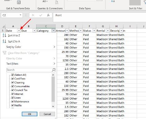
This will put an arrow on each column name that you can now click and view each unique value which can then be selected to only show data relating to that value.
Adding new columns with additional calculations for your bookings
You may want to add calculations to your booking costs to suit your needs, for example, deduct the 15% Booking.com charge or to add a cleaning fee.
You can do this by adding columns to the *.csv file and adding formulas that calculate the value for each row.
• Insert a column
> Highlight the column next to the “Costs” column > right click and Select “Insert”
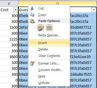
> Give the column a name and type the necessary formula in the first data row (below the column name).

>Press Enter

Examples of Formulas:
Deduct 15% fee:
= column * .85
e.g. =P2*0.85
Add $25 Cleaning fee:
= column + 25
e.g. =Q2+25
You now need to apply the formula to the remaining cells in that column.
You can do this by:
1. Dragging the formula from the top of the column to the bottom
> Hover over the lower right corner of the cell with the newly calculated value until you see a plus sign
> Click and drag the plus sign down until you get to the last cell in that column. Once you release the cursor, the formula will be applied to entire column
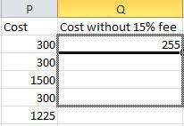
2. Copying the formula and pasting it to all the remaining cells of the column
> Select the data cell with the calculated value from the formula and Copy the value
> Select the empty cell below and drag the cursor until you get to the end of the column where you need data to be calculated then use your keyboard sequence e.g Ctrl P or mouse selection to Paste.
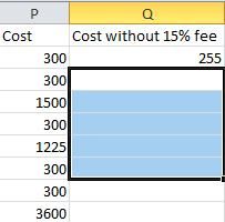
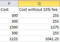
Once either of these methods is used, all of your rows should have the new column filled with the calculated values based on the formula.
Managing Spreadsheet data
Once you have the data there is any number of things you may want to do with it. Being able to manipulate the data to target your specific needs is a valuable skill that will serve you as a business owner. If you are new to working with spreadsheets please see the following resource which will guide you through the basics.